Lab 9: Hyperspectral Remote Sensing

Introduction

The goal of this lab is become a bit more familiar with ENVI software by using hyperspectral satellite images to perform some basic function in ENVI including atmospheric correction with FLAASH, vegetation index calculation, calculating agricultural stress, calculating the fire fuel, calculating forest health, and by performing a minimum noise fraction (MNF) transformation. Before these function were performed, hypersepctral statistics were looked at using a z-profile, and animation was created between bands.

Methods

View Hyperspectral Bands and Look at their Statistics

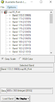Fig 1: Loading Hyperspectral Bands

This was done by opening up ENVI and loading a hyperspectral image in a viewer. Once the image was loaded. One is able to see the hundreds of bands which are available to be loaded. These bands can be seen at right in Figure 1. Next, regions of interest (ROI) were uploaded for the image using the restore ROIs function. Next, a plot was created for the ROIs. This plot was set to show the mean band reflectance and to display the minimum and maximum band reflectance values in the statistics immediately below it. This figure is shown in the results section.

Animate a Hyperspectral Image
In ENVI, animation can be created between bands. This is done by using the animation tool. Different parameters can be set to speed up or slow down the animation. Also, the area showing the animation can be edited.

Perform Atmospheric Correction
This was done using the FLAASH Atmospheric Correction tool. The parameters for this tool can be seen below in Figure 2. This tool resulted in an atmospherically corrected image.

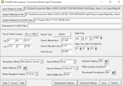Fig 2: Atmospheric Correction Parameters

After the image was corrected for, the original z-profile was compared with the corrected z-profile.

Calculate Vegetation Index

This was done by using the calculating vegetation index tool. Before entering in the parameters for this tool, a false color NIR band combination was loaded into a display.

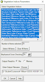Fig 3: Vegetation Index Paramters

This tool outputs many different images which show NDVI, simple ratio index, enhanced vegetation index, red edge normalized difference vegetation index, and many others.

Calculate Agricultural Stress

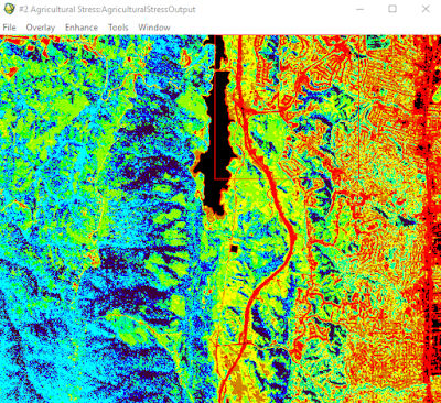
This was done using the agricultural stress tool.This tool is used to see where crops are stressed or not. This tool is used to see where plants are more efficient than others in using their available nitrogen, light, and moisture.

Calculate Fire Fuel

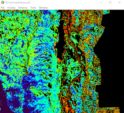
This was down using the Fire Fuel tool. This tool uses the NDVI index and the water band index to see where there is the most available fuel if a forest fire occurred. For this tool, because it'd be unnecessary to include urban areas, these areas were masked out using a mask. The parameters for this tool can be seen below in Figure 4.

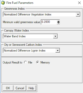Fig 4: Fire Fuel Parameters

Calculate Forest Health

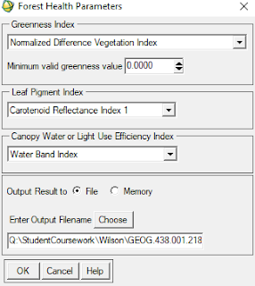
This was done using the Forest Health tool. The parameters for this tool can be seen below in Figure 5. This tool is uses the distribution of green vegetation, the concentration of stress for leaf pigments, the concentration of water in the forest canopy, and forest growth rates to create an overall forest's health.

Fig 5: Forest Health Parameters

Perform Minimum Noise Fraction (MNF) Transformation

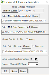
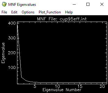
This was done by using the Estimate Noise Statistics From Data. The parameters for this MNF transformation can be seen below in Figure 6. To make the transformation be performed quicker, only the 20 bands between wavelengths 2.04 and 2.439 were used in the calculation. Also, the transformation was only performed on a small (20 x 20 pixel) subset of the original image.

Fig 6: MNF Parameters

Results

Figure 7 shows the animation created. This animation loops through bands 197 to 216 of the hyperspectral image. One can see how the bands all appear slightly different in this short video.

Fig 7: Animation Video

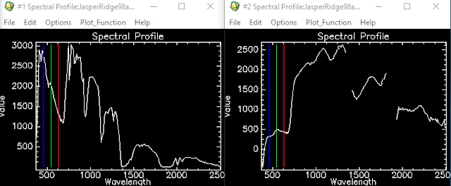
Figure 8 compares the results of the vegetation z-profile from the image that was atmospherically corrected to the image that wasn't. The corrected images profile is shown on the right while the original image's profile is shown on the left. One can see that the corrected image's profile looks as it normally should while the the original image's profile does not.

Fig 8: Comparing Vegetation Spectral Profiles

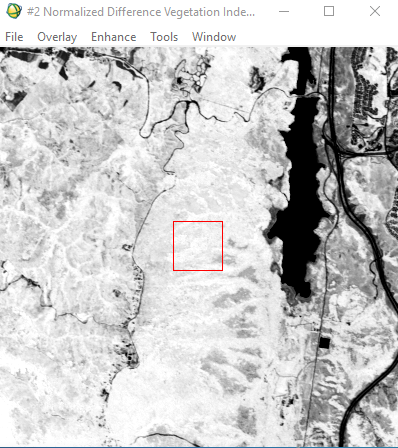
Figure 9 shows the NDVI image produced by running the Calculate Vegetation Index tool. This image shows that NDVI is high in the west and low in the east. This is because a forest resides in the western part of the image while a city resides in the eastern part of the image.

Fig 9: NDVI Image

Figure 10 shows the Simple Ratio Index also calculated by the Calculate Vegetation Index tool. This result shows that high values are located in the middle of the image while lower values are on  the outskirts.

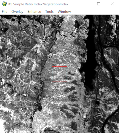Fig 10: Simple Ratio Index Image

Figure 11 shows the results of the Red Edge Normalized Vegetation Difference Index also calculated by the Calculate Vegetation Index tool. This is pretty much a normalized NDVI image. This image shows that the healthiest vegetation is in the southern middle part of the image while poor vegetation health is in the eastern part of the image where the town is located. This is because of roads and man-made features.

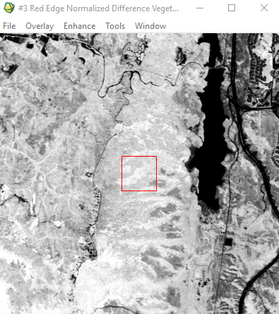Fig 11: Red Edge Normalized Vegetation Difference Index Image

Figure 12 shows the result of Agricultural Stress tool. It appears the most of the forest which is located in the western part of the image isn't stressed while, the vegetation located in the urban town is pretty stressed.

Figure 12: Agricultural Stress Output

Figure 13 shows the result of the Fire Fuel tool. Most of the fire fuel seems to be located around roads in the urban area which isn't much of a concern. The forest looks fairly moist which means that the fire fuel value is low.

Fig 13: Fire Fuel Output

Figure 14 shows the result of the Forest Health tool. This image shows that the forest health is very good across the forested area and is poor in the urban area. Red areas represent healthy forest while blue/purple areas represent an unhealthy forest. Based on this, the forest appears very healthy in the southwestern part, and moderately healthy in western part of the image.

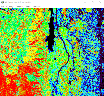Fig 14: Forest Health Output

Figure 15 shows the result of the MNF transformation's plot. The is an exponential inverse relationship between the eigenvalue and the eiganvalue number. A low egenvalue number will have a high eigenvalue, while a high eigenvalue number will have a low eiganvalue.

Fig 15: MNF Transformation Plot

Sources

ENVI, 2017. ENVI basic and Advanced Hyperspectral Analysis dataset
      http://www.harrisgeospatial.com/Support/SelfHelpTools/Tutorials.aspx
Wilson, C (2017) Lab 9 Hyperspectral Remote Sensing retrieved from
      https://drive.google.com/open?id=1tLLd6zyeLqslKT3heVtu19qtmNuZQisK