Lab 8: Classifying Imagery With the Expert System and ENVI

Introduction

The first goal of this lab is to improve image classification accuracy using the expert system in Erdas ancillary zoning and other data of the Eau Claire and Chippewa area. The second goal is to perform artificial neural network image classification of Northern Iowa's campus using ENVI software. the expert system is the best of the image classification systems as it uses ancillary data such as elevation, demographics, income, and zoning to refine an already classified image. Using the expert system has been used to generate accuracy as high as 94%. In this lab, only qualitative assessment will be performed. Also, a map of the classified image will be created.

Methods

Using the Expert Classification System
The expert classification is more of a reclassification than it is a classification. This is because to use the expert classification system one needs to already have a classified image. In this lab a classified image of Eau Claire and Chippewa area was used. This classified image had many incorrectly classified areas. These areas mainly included golf courses, cemeteries are other urban areas.

Set up the Knowledge Engineer
The Knowledge Engineer is the interface for which the expert system is used in. It can be opened by navigating to Raster → Knowledge Engineer → Knowledge Engineer. The Knowledge Engineer window can be seen below in Figure 1.

Fig 1: Knowledge Engineer Window

In the window, hypotheses, rules, and variables are added to help reclassify the imagery. Hypotheses appear in green, rules appear in yellow, and variables appear in blue.

Each rule applies to ancillary data. For example, an area that is classified for agriculture in the original image, but is in a zoning class of residential, the classification for areas that are classified as agriculture in residential areas can be changed from agriculture to urban by assigning rules.

An example of a rule can be seen below in Figure 2. For the input raster (ancillary data) which is assigned to the variable GV_agric. When, this variable has a class value of 1, the classified image cannot have that pixel be assigned to a value of 4. For pixels which are assigned a pixel value of 4, their values are changed to 1.

Fig 2: Rule for Agriculture

Similar rules like this were written for urban, residential, green vegetation and other urban classes. The hypotheses, rules, and variables for these can be seen below in Figure 3.

Fig 3: Hypotheses, Rules, and Variables Used

Perform the Classification
To run the expert classification, one can click navigate to the Knowledge Classifier window. The classification scheme which is set up above is brought in. Then, the next button is clicked. Then, some parameters are changed so that the "set window" is changed from Intersect to Union. This can be seen below in Figure 4. The Set Window window is open by clicking on the Set... button. Then, the output is specified and the tool is ran.

Fig 4: Running the Classification

Lastly, a map of the output is created in ArcMap.

Using ENVI to Classify Imagery
Neural network classification imitates the way a human would classify imagery. It uses ancillary data along with weights and hidden layers to classify the imagery. To perform neural network classification in ENVI, first the image of the University of Northern Iowa's campus is loaded into a viewer. The band combination is set to NIR, Red , Green as this is a typical band combination for classifying imagery.

Then, training samples are collected (called ROI's in ENVI) by using the #ROI Tool window. This window with the filled training samples can be seen below in Figure 5.

Fig 5: Collected ROIs (Training Samples)

Next these training samples are used to help run the classification. This is done by navigating to Classification → Supervised → Neural Net on the main toolbar. Then, in the Neural Net Parameters window, the parameters are changed to set the training rate, training momentum, and the number of training iterations. Each of these parameters will affect how the image will be classified. Lastly, the output is saved to a folder.

The classification was ran a few times with each time altering the number of iterations to see how the number of iterations affects the classification of the imagery.

Results

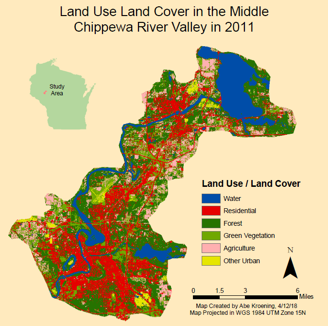
Figure 6 shows the map created in ArcMap of the classified system using the expert system. Areas that changed the most from the original classified image include cemeteries, golf courses, and other urban areas such as the mall and sand mines. The class "other urban" was created because zoning data was used to help classify the imagery. If the zoning data was residential, then areas classified as urban were classified as other urban. This is why areas such as the airport, the mall, and industrial complexes are classified as other urban.

Fig 6: LULC Map Created Using the Expert System

Figure 7 shows the results of the neural classification performed in ENVI using 100 iterations. The red areas represent roofs, the blue areas represent green vegetation, and the green areas represent asphalt ans sidewalks.

Fig 7: Neural Network Classification

Figure 8 shows the results of comparing the number of iterations. To help see the differences, only a small portion of the campus is pictured at a very large scale. It appears that the image with more iterations is slightly smoother than the image which was produced using fewer iterations. This can be see by comparing the roof tops located on the right side of each image. Although, the output is smoother, the more iterations that are ran, the longer it takes to produce the output image.

Fig 8: Comparing the Number of Iterations

Sources

United States Geological Survey, (2017). Earth Resources Observation and Science Center
University of Northern Iowa Geography Department (2016) Quickbird High resolution imagery
Wilson, C (2017) Lab 8 Expert System Classification retrieved from
    https://drive.google.com/file/d/15fOh_xcupGKzPqZixYQguXm3yex0VJDa/view?usp=sharing